Cookbook

library(reactablefmtr)
library(htmltools)
library(tidyverse)

Overview

A high-level overview of the functions and styling customization options available in {reactablefmtr}.

Titles and Sources

A title, subtitle, and source can be added to any reactable table using add_title(), add_subtitle(), and add_source() respectively. There are several built-in formatters available, such as the ability to change the font size, font color, font style, and margin.

library(palmerpenguins)

reactable(penguins) %>% 
  add_title(
    title = 'Palmer Penguins'
  ) %>% 
  add_subtitle(
    subtitle = 'Palmer Archipelago (Antarctica) penguin data',
    font_size = 20,
    font_color = '#666666',
    margin = reactablefmtr::margin(t=10,r=0,b=15,l=0)
  ) %>% 
  add_source(
    source = 'Authors: Allison Marie Horst, Alison Presmanes Hill, and Kristen B Gorman',
    font_style = 'italic',
    font_weight = 'bold'
  )

Palmer Penguins

Palmer Archipelago (Antarctica) penguin data

Authors: Allison Marie Horst, Alison Presmanes Hill, and Kristen B Gorman

Inserting images and icons

You can also parse HTML with reactablefmtr::html(). This allows for the ability to add images and clickable links within the title and source as shown below:

reactable(penguins) %>% 
  add_title(
    title = reactablefmtr::html("Palmer Penguins <img src='https://raw.githubusercontent.com/allisonhorst/palmerpenguins/master/man/figures/lter_penguins.png' alt='Palmer Penguins' width='200' height='110'>")
  ) %>% 
  add_subtitle(
    subtitle = 'Palmer Archipelago (Antarctica) penguin data',
    font_size = 20,
    font_color = '#666666',
    margin = reactablefmtr::margin(t=10,r=0,b=15,l=0)
  ) %>% 
  add_source(
    source = reactablefmtr::html("<i class='fas fa-book'></i> Authors: Allison Marie Horst, Alison Presmanes Hill, and Kristen B Gorman <br> <i class='fas fa-palette'></i> Artwork by @allison_horst "),
    font_style = 'italic',
    font_weight = 'bold'
  ) %>% 
  add_source(
    source = html("<i class='fas fa-link'></i> Link to package: <a href='https://allisonhorst.github.io/palmerpenguins/'>{palmerpenguins}</a>"),
    font_style = 'italic',
    font_weight = 'bold'
  )

Palmer Penguins

Palmer Archipelago (Antarctica) penguin data

Authors: Allison Marie Horst, Alison Presmanes Hill, and Kristen B Gorman
Artwork by @allison_horst

Link to package: {palmerpenguins}

Themes

There are over 20 themes available within {reactablefmtr} that can be applied simply within reactable::theme.

There are additional styling options within each theme that allows you to change the font color and font size of both the body of the table and the header, as shown below in the NY Times-inspired table:

Another important feature within each theme is the ability to vertically center the values within each row. By default, {reactable} tables display the values towards the top of each cell. To center the values, include centered = TRUE within the theme options:

FiveThirtyEight

penguins %>% 
  reactable(theme = fivethirtyeight()) 

New York Times

penguins %>% 
  reactable(theme = nytimes()) 

Dark

penguins %>% 
  reactable(theme = dark())

Bootsrap Themes

penguins %>% 
  reactable(theme = superhero()) 

Bubble grids

Bubble grid charts can easily be created with the bubble_grid() function:

penguins %>%
  group_by(species, sex) %>%
  summarize(across(where(is.numeric), mean, na.rm = TRUE)) %>%
  select(-year) %>%
  reactable(
    defaultColDef = colDef(
      align = 'center',
      cell = bubble_grid(
        data = .,
        number_fmt = scales::comma
      )
    )
  )

Adjust size of bubbles

Adjust the size of the bubbles using min_value and/or max_value:

# load bee colony stressor dataset from tidy tuesday 
stressor <- readr::read_csv('https://raw.githubusercontent.com/rfordatascience/tidytuesday/master/data/2022/2022-01-11/stressor.csv')

stressor %>% 
  filter(year == 2020 & state %in% c('United States','California','Georgia','Texas','Idaho')) %>%
  group_by(state, stressor) %>% 
  summarize(stress_pct = mean(stress_pct, na.rm = TRUE)) %>% 
  pivot_wider(names_from = stressor, values_from = stress_pct) %>% 
  select(c(State = state, Diseases = Disesases, Pesticides, `Other pests/parasites`, Other, Unknown)) %>%
  reactable(
    theme = no_lines(centered = TRUE),
    defaultColDef = colDef(align = 'center'),
    columns = list(
      Diseases = colDef(
        cell = bubble_grid(
          data = .,
          colors = '#084C61',
          number_fmt = scales::number,
          min_value = 0,
          max_value = 15
        )
      ), 
      Pesticides = colDef(
        cell = bubble_grid(
          data = .,
          colors = '#DB504A',
          number_fmt = scales::number,
          min_value = 0,
          max_value = 15
        )
      ), 
      `Other pests/parasites` = colDef(
        cell = bubble_grid(
          data = .,
          colors = '#E3B505',
          number_fmt = scales::number,
          min_value = 0,
          max_value = 15
        )
      ),
      Other = colDef(
        cell = bubble_grid(
          data = .,
          colors = '#4F6D7A',
          number_fmt = scales::number,
          min_value = 0,
          max_value = 15
        )
      ), 
      Unknown = colDef(
        cell = bubble_grid(
          data = .,
          colors = '#56A3A6',
          number_fmt = scales::number,
          min_value = 0,
          max_value = 15
        )
      )
    )
  ) %>% 
  add_title(
    title = reactablefmtr::html("Bee Colony Health Stressors <img src='https://svgsilh.com/svg/30649.svg' alt='Bee' width='40' height='40'>"),
    margin = reactablefmtr::margin(t=0,r=0,b=3,l=0)
    ) %>% 
  add_subtitle(
    subtitle = '% of colonies affected by stressors during 2020',
    font_weight = 'normal',
    font_size = 20,
    margin = reactablefmtr::margin(t=0,r=0,b=6,l=0)
    ) %>% 
  add_source(
    source = 'Data: USDA, #TidyTuesday Week 2, 2022',
    margin = reactablefmtr::margin(t=7,r=0,b=0,l=0),
    font_style = "italic"
    )

Bee Colony Health Stressors

% of colonies affected by stressors during 2020

Data: USDA, #TidyTuesday Week 2, 2022

Note that the animation on sort disappears when the bubbles are all the same color in each column. This is because, by default, the color of the bubble is the only element set to animate on sort, which is set by animation = background 1s ease'. If you still want to see some sort of animation, you could set the animation property to ‘all 1s ease’ as shown below:

If you’re interested in learning more about animation options, please see the CSS transition property documentation here.

Bubble squares

In addition to bubble circles, you can also create bubble squares by setting the shape parameter to ‘squares’:

penguins %>%
  group_by(species, sex) %>%
  summarize(across(where(is.numeric), mean, na.rm = TRUE)) %>%
  select(-year) %>%
  reactable(
    theme = no_lines(centered = TRUE),
    defaultColDef = colDef(align = 'center'),
    columns = list(
      bill_length_mm = colDef(
        cell = bubble_grid(
          data = .,
          shape = 'squares',
          colors = c('#f2f0f7','#cbc9e2','#9e9ac8','#756bb1','#54278f'),
          box_shadow = TRUE,
          number_fmt = scales::number_format(accuracy = 0.1),
          min_value = 30,
          animation = 'all 1s ease'
        )
      ),
      bill_depth_mm = colDef(
        cell = bubble_grid(
          data = .,
          shape = 'squares',
          colors = c('#feedde','#fdbe85','#fd8d3c','#e6550d','#a63603'),
          box_shadow = TRUE,
          number_fmt = scales::number_format(accuracy = 0.1),
          min_value = 13,
          max_value = 21,
          animation = 'all 1s ease'
        )
      ),
      flipper_length_mm = colDef(
        cell = bubble_grid(
          data = .,
          shape = 'squares',
          colors = c('#f1eef6','#bdc9e1','#74a9cf','#2b8cbe','#045a8d'),
          box_shadow = TRUE,
          number_fmt = scales::number_format(accuracy = 0.1),
          min_value = 120,
          animation = 'all 1s ease'
        )
      ),
      body_mass_g = colDef(
        cell = bubble_grid(
          data = .,
          shape = 'squares',
          colors = c('#edf8e9','#bae4b3','#74c476','#31a354','#006d2c'),
          opacity = 0.8,
          box_shadow = TRUE,
          number_fmt = scales::comma,
          min_value = 2000,
          animation = 'all 1s ease'
        )
      )
    )
  )

Bar charts

There are many ways to customize the appearance of the bar charts within data_bars():

penguins %>% 
  group_by(species, island, sex) %>% 
  summarize(across(where(is.numeric), mean, na.rm = TRUE)) %>% 
  select(-year) %>% 
  reactable(
    theme = clean(),
    pagination = FALSE,
    columns = list(
      bill_length_mm = colDef(
        cell = data_bars(
          data = .,
          fill_color = viridis::mako(5),
          background = '#F1F1F1',
          min_value = 35,
          max_value = 55,
          text_position = 'outside-end',
          number_fmt = scales::comma
        )
      ),
      bill_depth_mm = colDef(
        cell = data_bars(
          data = .,
          fill_color = c('#FFF2D9','#FFE1A6','#FFCB66','#FFB627'),
          fill_gradient = TRUE,
          background = 'transparent',
          number_fmt = scales::comma_format(accuracy = 0.1)
        )
      ),
      flipper_length_mm = colDef(
        cell = data_bars(
          data = .,
          fill_color = 'black',
          fill_opacity = 0.8,
          round_edges = TRUE,
          text_position = 'center',
          number_fmt = scales::comma
        )
      ),
      body_mass_g = colDef(
        cell = data_bars(
          data = .,
          fill_color = 'white',
          background = 'darkgrey',
          border_style = 'solid',
          border_width = '1px',
          border_color = 'forestgreen',
          box_shadow = TRUE,
          text_position = 'inside-base',
          number_fmt = scales::comma
        )
      )
    )
  )

Conditional fill

Conditionally assign colors to bars by assigning the colors within a new column using dplyr::case_when() and then referencing that column to be used as the fill of the bars with fill_color_ref:

survey <- data.frame(
  response = c('Agree','Disagree','Neutral'),
  percentage = c(0.64, 0.29, 0.07)
)

survey %>% 
  mutate(response_colors = case_when(
    response == 'Agree' ~ '#127852',
    response == 'Disagree' ~ '#C40233',
    TRUE ~ '#A5A0A1'
  )) %>% 
  reactable(
    theme = clean(centered = TRUE),
    columns = list(
      response_colors = colDef(show = FALSE),
      response = colDef(maxWidth = 110),
      percentage = colDef(
        align = 'left',
        cell = data_bars(
          data = .,
          fill_color_ref = 'response_colors',
          number_fmt = scales::percent,
          max_value = 1,
          bar_height = 50,
          text_size = '1.3em'
        )
      )
    )
  )

Fill by another column

Alternatively, you can use fill_by to apply a bar chart to a column containing text:

survey %>%
  mutate(response_colors = case_when(
    response == 'Agree' ~ '#127852',
    response == 'Disagree' ~ '#C40233',
    TRUE ~ '#8C8687'
  ),
  response = paste0(response, " (", percentage*100, "%)")) %>%
  reactable(
    theme = void(centered = TRUE),
    columns = list(
      response = colDef(
        name = '',
        cell = data_bars(
          data = .,
          fill_by = 'percentage',
          fill_color_ref = 'response_colors',
          text_position = 'outside-end',
          max_value = 1,
          bar_height = 50,
          text_color_ref = 'response_colors',
          text_size = '1.5em',
          bold_text = TRUE
        )
      ),
      response_colors = colDef(show = FALSE),
      percentage = colDef(show = FALSE)
    )
  ) %>%
  add_title('Survey Responses')

Survey Responses

Add icons to bars

If you would like to add an icon to the data bars, you can do so by providing the name of the icon within the icon parameter.

Note that the color of the icon will automatically be inherited by the color of the data bar unless provided explicity within the icon_color parameter.

cars <- mtcars %>%
  rownames_to_column(var = 'model') %>% 
  select(c(model,mpg,hp)) 

reactable(cars,
  theme = nytimes(centered = TRUE),
  compact = TRUE,
  defaultSortOrder = 'desc',
  defaultSorted = 'hp',
  pagination = FALSE,
  columns = list(
    hp = colDef(
      minWidth = 150,
      cell = data_bars(
        data = cars,
        text_position = 'none',
        box_shadow = TRUE,
        round_edges = TRUE,
        fill_color = rev(MetBrewer::met.brewer('Troy')),
        bias = 1.5,
        icon = 'horse-head',
        background = 'transparent',
        bar_height = 4,
        max_value = 400
      )
    ),
    mpg = colDef(
      minWidth = 150,
      cell = data_bars(
        data = cars,
        text_position = 'none',
        box_shadow = TRUE,
        round_edges = TRUE,
        fill_color = MetBrewer::met.brewer('VanGogh3'),
        bias = 1.5,
        icon = 'leaf',
        background = 'transparent',
        bar_height = 4
      )
    )
  )
) 

Adding images to bars

To add an external web image to the data bars, you can do so by providing a link to the image within the img parameter:

cars <- mtcars %>%
  rownames_to_column(var = 'model') %>%
  select(c(model,mpg,cyl,drat,wt,hp,qsec)) %>%
  mutate(rank = rank(qsec)) %>%
  relocate(rank, .before = 'model')

reactable(cars,
  theme = nytimes(centered = TRUE, font_color = '#666666'),
  compact = TRUE,
  defaultSortOrder = 'asc',
  defaultSorted = 'qsec',
  pagination = FALSE,
  showSortIcon = FALSE,
  columns = list(
    model = colDef(
      minWidth = 100,
      style = cell_style(
        data = cars,
        font_color = '#222222',
        font_weight = 'bold'
      )),
    mpg = colDef(maxWidth = 60),
    cyl = colDef(maxWidth = 60),
    hp = colDef(maxWidth = 60),
    drat = colDef(maxWidth = 60),
    wt = colDef(maxWidth = 60),
    rank = colDef(
      maxWidth = 45,
      format = colFormat(digits = 0)
    ),
    qsec = colDef(
      name = '1/4 mile time',
      align = 'left',
      minWidth = 200,
      format = colFormat(digits = 0),
      cell = data_bars(
        data = cars,
        fill_color = c('#FAFAFA','#E7E7E7','#D3D3D3','#BFBFBF'),
        fill_gradient = TRUE,
        bold_text = TRUE,
        background = 'transparent',
        text_position = 'inside-base',
        text_color = '#222222',
        number_fmt = scales::number_format(accuracy = 0.1, suffix = 's'),
        bar_height = 12,
        min_value = 13,
        max_value = 25,
        img = 'https://www.pngkit.com/png/detail/54-544889_45-top-view-of-car-clipart-images-racecar.png',
        img_height = 20,
        img_width = 25
      )
    )
  )
) %>%
  add_title(
    title = reactablefmtr::html("Fastest cars in the mtcars dataset <i class='fas fa-flag-checkered'></i>"),
    font_color = 'black',
    text_shadow = '1px 1px 2px red',
    margin = margin(t=0,r=0,b=5,l=0)
  )

Fastest cars in the mtcars dataset

Display positive and negative values

Data bars are able to display both positive and negative values automatically:

cars <- mtcars %>%
  rownames_to_column(var = 'model') %>% 
  select(c(model,wt,mpg,hp)) %>% 
  mutate(wt = wt-mean(wt),
         mpg = mpg-mean(mpg),
         hp = hp-mean(hp))

reactable(cars,
  theme = nytimes(centered = TRUE),
  compact = TRUE,
  defaultSortOrder = 'desc',
  defaultSorted = 'mpg',
  pagination = FALSE,
  columns = list(
    wt = colDef(
      name = 'WT VS AVG',
      minWidth = 150,
      align = 'center',
      cell = data_bars(
        data = cars,
        text_position = 'outside-end',
        fill_color = viridis::mako(5),
        number_fmt = scales::number_format(accuracy = 0.01)
      )
    ),
    hp = colDef(
      name = 'HP VS AVG',
      minWidth = 150,
      align = 'center',
      cell = data_bars(
        data = cars,
        text_position = 'outside-end',
        fill_color = c('#C40233','#127852'),
        number_fmt = scales::comma
      )
    ),
    mpg = colDef(
      name = 'MPG VS AVG',
      minWidth = 150,
      align = 'center',
      cell = data_bars(
        data = cars,
        text_position = 'none',
        box_shadow = TRUE,
        fill_color = MetBrewer::met.brewer('VanGogh3'),
        number_fmt = scales::comma
      )
    )
  )
) 

Dot plots

You can create dot plot charts by assigning a ‘circle’ icon to the data bars and making the data bars transparent:

midwest %>% 
  group_by(state, county) %>% 
  summarize(perchsd = mean(perchsd/100, na.rm = TRUE),
            percollege = mean(percollege/100, na.rm = TRUE)) %>% 
  filter(state == 'IL') %>% 
  reactable(
  theme = clean(),
  defaultSorted = 'county',
  defaultPageSize = 25,
  paginationType = 'jump',
  columns = list(
    state = colDef(maxWidth = 80),
    county = colDef(maxWidth = 120),
    perchsd = colDef(
      name = '% with a High School Diploma',
      align = 'left',
      minWidth = 250,
      cell = data_bars(
        data = .,
        fill_color = '#EEEEEE',
        number_fmt = scales::percent,
        text_position = 'outside-end',
        max_value = 1,
        icon = 'circle',
        icon_color = 'firebrick',
        icon_size = 15,
        text_color = 'firebrick',
        round_edges = TRUE
      )
    ),
    percollege = colDef(
      name = '% with a College Education',
      align = 'left',
      minWidth = 250,
      cell = data_bars(
        data = .,
        fill_color = '#EEEEEE',
        number_fmt = scales::percent,
        text_position = 'outside-end',
        max_value = 1,
        icon = 'circle',
        icon_color = '#226ab2',
        icon_size = 15,
        text_color = '#226ab2',
        round_edges = TRUE
      )
    )
  )
)

Lollipop charts

You can create lollipop charts by following a similar method used to create the dot plot charts above, but by adding color to the data bars and reducing the height of the bars:

midwest %>% 
  group_by(state, county) %>% 
  summarize(perchsd = mean(perchsd/100, na.rm = TRUE),
            percollege = mean(percollege/100, na.rm = TRUE)) %>% 
  filter(state == 'IL') %>% 
  reactable(
  theme = clean(),
  defaultSorted = 'county',
  defaultPageSize = 25,
  paginationType = 'jump',
  columns = list(
    state = colDef(maxWidth = 80),
    county = colDef(maxWidth = 120),
    perchsd = colDef(
      name = '% with a High School Diploma',
      align = 'left',
      minWidth = 250,
      cell = data_bars(
        data = .,
        fill_color = 'firebrick',
        background = '#FFFFFF',
        bar_height = 7,
        number_fmt = scales::percent,
        text_position = 'outside-end',
        max_value = 1,
        icon = 'circle',
        icon_color = 'firebrick',
        icon_size = 15,
        text_color = 'firebrick',
        round_edges = TRUE
      )
    ),
    percollege = colDef(
      name = '% with a College Education',
      align = 'left',
      minWidth = 250,
      cell = data_bars(
        data = .,
        fill_color = '#226ab2',
        background = '#FFFFFF',
        bar_height = 7,
        number_fmt = scales::percent,
        text_position = 'outside-end',
        max_value = 1,
        icon = 'circle',
        icon_color = '#226ab2',
        icon_size = 15,
        text_color = '#226ab2',
        round_edges = TRUE
      )
    )
  )
)

Heatmaps

Heatmaps can be created by using the color_scales() function and hiding the text by setting show_text to FALSE. Additionally, you can set tooltip to TRUE so that you can still see the values when a user hovers over each cell:

sanmarcos_sales <- txhousing %>% 
  filter(city == 'San Marcos' & year > 2004 & year < 2015) %>%
  group_by(year, month) %>% 
  summarize(sales = mean(sales, na.rm = TRUE)) %>%
  mutate(month = month.abb[month]) %>% 
  pivot_wider(names_from = 'month', values_from = 'sales') %>% 
  ungroup() %>% 
  mutate(year = as.character(year),
         total = rowSums(across(where(is.numeric))))

sanmarcos_legend <- txhousing %>% 
  filter(city == 'San Marcos' & year > 2004 & year < 2015) %>%
  group_by(year, month) %>% 
  summarize(sales = mean(sales, na.rm = TRUE)) %>%
  mutate(month = month.abb[month]) 

reactable(
  sanmarcos_sales,
  pagination = FALSE,
  showSortIcon = FALSE,
  theme = void(
    centered = TRUE, 
    cell_padding = 0,
    header_font_color = 'black',
    font_color = 'black'
    ),
  defaultColDef = colDef(
    maxWidth = 50,
    align = 'center',
    cell = tooltip(),
    style = color_scales(
      data = sanmarcos_sales,
      span = 2:13,
      colors = c('#002347','#003366','#003F7D','#FF8E00','#FD7702','#FF5003'),
      bias = 1.4,
      opacity = 0.9,
      show_text = FALSE
    )
  ),
  columns = list(
    total = colDef(
      maxWidth = 225,
      cell = data_bars(
        data = sanmarcos_sales,
        fill_color = c('#002347','#003366','#003F7D','#FF8E00','#FD7702','#FF5003'),
        bias = 1.4,
        fill_opacity = 0.9,
        background = 'transparent',
        bar_height = 40,
        text_position = 'center'
        ),
      style = list(borderLeft = "2px solid #999999")
    )
  )
) %>% 
  add_title(
    title = html("San Marcos Housing Sales <i class='fas fa-home'></i>"),
    align = 'center',
    margin = reactablefmtr::margin(t=10,r=0,b=2,l=0)
  ) %>% 
  add_subtitle(
    subtitle = 'Hover over cells to see values',
    font_style = 'italic',
    font_color = '#777777',
    font_size = 18,
    align = 'center',
    margin = reactablefmtr::margin(t=0,r=0,b=10,l=0)
  ) %>% 
  add_legend(
    data = sanmarcos_legend,
    align = 'left',
    title = '# of Sales (Jan - Dec)',
    col_name = 'sales',
    colors = c('#002347','#003366','#003F7D','#FF8E00','#FD7702','#FF5003'),
    bias = 1.4,
    bins = 6
  )

San Marcos Housing Sales

Hover over cells to see values

# of Sales (Jan - Dec)

• 6

• 14

• 19

• 26

• 34

• 63

Nested tables

{reactablefmtr} styling supports nested {reactable} tables that expand on click:

data <- MASS::Cars93[1:30, c('Type','Make','Model','MPG.city','MPG.highway')]

averages <- data %>%
  group_by(Type) %>%
  summarize(
    MPG.city = mean(MPG.city),
    MPG.highway = mean(MPG.highway)
  )

reactable(
  averages,
  theme = clean(centered = TRUE),
  columns = list(
    Type = colDef(maxWidth = 250),
    MPG.city = colDef(
      maxWidth = 200, 
      style = color_scales(
        data = data, 
        colors = viridis::mako(5)), 
      format = colFormat(digits = 1)),
    MPG.highway = colDef(
      maxWidth = 200, 
      cell = data_bars(
        data = data, 
        fill_color = viridis::mako(5), 
        number_fmt = scales::comma))
    ),
  onClick = "expand",
  details = function(index) {
    data_sub <- data[data$Type == averages$Type[index], ]
    reactable(
      data_sub,
      theme = clean(centered = TRUE),
      columns = list(
        Type = colDef(show = FALSE),
        Make = colDef(maxWidth = 175),
        Model = colDef(maxWidth = 120),
        MPG.city = colDef(
          maxWidth = 200, 
          style = color_scales(data, viridis::mako(5)), 
          format = colFormat(digits = 1)),
        MPG.highway = colDef(
          maxWidth = 200, 
          cell = data_bars(data, fill_color = viridis::mako(5), number_fmt = scales::comma))
        )
    ) 
  }
)

Pill buttons

Pill buttons can be applied to both numeric and character values. By default, a single color will be applied across all values, but the colors can be assigned via another column within the color_ref parameter:

data <- tribble(
  ~name,~date,~location,~units,~amount,~avg_unit,~status,~colors,
  'John','2022-03-05','Seattle',40,10000,250,'Approved','lightgreen',
  'Jane','2022-04-01','Denver',20,15000,750,'Pending Approval','gold1',
  'Luke','2022-03-31','Austin',15,8000,533,'Approved','lightgreen',
  'Mary','2022-03-28','New York',25,21000,840,'Cancelled','lightpink',
  'Peter','2022-04-05','Miami',10,17000,1700,'Pending Approval','gold1',
  'Paul','2022-03-22','Los Angeles',30,12000,400,'Approved','lightgreen'
  )

data %>% 
  reactable(
    theme = pff(centered = TRUE),
    defaultColDef = colDef(footerStyle = list(fontWeight = "bold")),
    columns = list(
      name = colDef(
        minWidth = 175,
        footer = 'Total',
        cell = merge_column(
          data = .,
          merged_name = 'location',
          merged_position = 'below',
          merged_size = 14,
          size = 16,
          color = '#333333',
          spacing = -1
        )
      ),
      date = colDef(
        minWidth = 125,
        cell = pill_buttons(
          data = .,
          opacity = 0.8
        )
      ),
      location = colDef(show = FALSE),
      units = colDef(footer = function(values) scales::label_number()(sum(values))),
      amount = colDef(
        cell = function(value) {scales::label_dollar()(value)},
        footer = function(values) scales::label_dollar()(sum(values))),
      avg_unit = colDef(
        name = 'Avg/Unit', 
        cell = function(value) scales::label_dollar()(value),
        footer = function(values) scales::label_dollar()(mean(values))),
      status = colDef(
        minWidth = 175,
        cell = pill_buttons(
          data = .,
          color_ref = 'colors',
          box_shadow = TRUE
        )
      ),
      colors = colDef(show = FALSE)
    )
  ) %>% 
  add_title(
    title = 'Client Order Summary'
  )

Client Order Summary

Color tiles

Color tiles provide an alternative to pill buttons and color scales with many customization options available.

library(viridis)

penguins %>%
  group_by(species, island, sex) %>%
  summarize(across(where(is.numeric), mean, na.rm = TRUE)) %>%
  mutate(penguin_colors = case_when(
    species == 'Adelie' ~ '#F5A24B',
    species == 'Chinstrap' ~ '#AF52D5',
    species == 'Gentoo' ~ '#4C9B9B',
    TRUE ~ 'grey'
  )) %>% 
  select(-c(year,flipper_length_mm)) %>%
  reactable(
    columns = list(
      species = colDef(
        cell = color_tiles(
          data = .,
          color_ref = 'penguin_colors'
        )
      ),
      bill_length_mm = colDef(
        cell = color_tiles(
          data = .,
          number_fmt = scales::comma
        )
      ),
      bill_depth_mm = colDef(
        cell = color_tiles(
          data = .,
          colors = viridis::mako(5),
          number_fmt = scales::comma_format(accuracy = 0.1)
        )
      ),
      body_mass_g = colDef(
        cell = color_tiles(
          data = .,
          colors = c('#011936','#465362','#82A3A1','#9FC490','#C0DFA1'),
          number_fmt = scales::comma,
          opacity = 0.7,
          bold_text = TRUE,
          box_shadow = TRUE
        )
      ),
      penguin_colors = colDef(show = FALSE)
    )
  )

Sparklines

Use react_sparkline() to create sparkline charts from values stored in a list:

penguins %>%
  group_by(species, island) %>%
  na.omit(.) %>% 
  summarize(across(where(is.numeric), list)) %>%
  mutate(penguin_colors = case_when(
    species == 'Adelie' ~ '#F5A24B',
    species == 'Chinstrap' ~ '#AF52D5',
    species == 'Gentoo' ~ '#4C9B9B',
    TRUE ~ 'grey'
  )) %>% 
  select(-c(year,body_mass_g,flipper_length_mm)) %>% 
reactable(
  .,
  theme = pff(centered = TRUE),
  compact = TRUE,
  columns = list(
    species = colDef(maxWidth = 90),
    island = colDef(maxWidth = 85),
    penguin_colors = colDef(show = FALSE),
    bill_length_mm = colDef(
      cell = react_sparkline(
        data = .,
        height = 100,
        line_width = 1.5,
        bandline = 'innerquartiles',
        bandline_color = 'forestgreen',
        bandline_opacity = 0.6,
        labels = c('min','max'),
        label_size = '0.9em',
        highlight_points = highlight_points(min = 'blue', max = 'red'),
        margin = reactablefmtr::margin(t=15,r=2,b=15,l=2),
        tooltip_type = 2
      )
    ),
    bill_depth_mm = colDef(
      cell = react_sparkline(
        data = .,
        height = 100,
        line_width = 1.5,
        bandline = 'innerquartiles',
        bandline_color = 'forestgreen',
        bandline_opacity = 0.6,
        labels = c('min','max'),
        label_size = '0.9em',
        highlight_points = highlight_points(min = 'blue', max = 'red'),
        margin = reactablefmtr::margin(t=15,r=2,b=15,l=2),
        tooltip_type = 2
      )
    )
  )
)

Sparklines with area shown

You can display the area below the sparklines by setting the show_area formatter to TRUE:

penguins %>%
  group_by(species, island) %>%
  na.omit(.) %>% 
  summarize(across(where(is.numeric), list)) %>%
  mutate(penguin_colors = case_when(
    species == 'Adelie' ~ '#F5A24B',
    species == 'Chinstrap' ~ '#AF52D5',
    species == 'Gentoo' ~ '#4C9B9B',
    TRUE ~ 'grey'
  )) %>% 
  select(-c(year,body_mass_g,flipper_length_mm)) %>% 
  relocate(island, .before = 'species') %>% 
reactable(
  .,
  theme = dark(centered = TRUE),
  compact = TRUE,
  columns = list(
    species = colDef(
      align = 'center',
      maxWidth = 100,
        cell = pill_buttons(
          data = .,
          color_ref = 'penguin_colors',
          brighten_text = FALSE,
          bold_text = TRUE
        )
    ),
    island = colDef(maxWidth = 85),
    penguin_colors = colDef(show = FALSE),
    bill_length_mm = colDef(
      cell = react_sparkline(
        data = .,
        height = 100,
        show_area = TRUE,
        area_opacity = 1,
        line_color_ref = 'penguin_colors',
        labels = 'max',
        label_size = '1em',
        tooltip_type = 2
      )
    ),
    bill_depth_mm = colDef(
      cell = react_sparkline(
        data = .,
        height = 100,
        show_area = TRUE,
        area_opacity = 1,
        line_color_ref = 'penguin_colors',
        labels = 'max',
        label_size = '1em',
        tooltip_type = 2
      )
    )
  )
)

Sparkbars

Sparkbar charts can also be created by using the react_sparkbar() function. Many of the options that are available in react_sparkline() are also available in the sparkbars.

penguins %>%
  group_by(species) %>%
  na.omit(.) %>% 
  summarize(across(where(is.numeric), list)) %>%
  mutate(penguin_colors = case_when(
    species == 'Adelie' ~ '#F5A24B',
    species == 'Chinstrap' ~ '#AF52D5',
    species == 'Gentoo' ~ '#4C9B9B',
    TRUE ~ 'grey'
  )) %>% 
  select(-c(year,body_mass_g,bill_depth_mm, bill_length_mm)) %>% 
reactable(
  .,
  theme = dark(centered = TRUE),
  compact = TRUE,
  columns = list(
    species = colDef(
      name = 'Species',
      align = 'center',
      maxWidth = 160,
        cell = pill_buttons(
          data = .,
          color_ref = 'penguin_colors',
          text_size = 22,
          brighten_text = FALSE,
          bold_text = TRUE
        )
    ),
    penguin_colors = colDef(show = FALSE),
    flipper_length_mm = colDef(
      name = 'Flipper Length (mm)',
      align = 'center',
      cell = react_sparkbar(
        data = .,
        height = 160,
        fill_color_ref = 'penguin_colors',
        statline = 'median',
        statline_color = '#FFFFFF',
        statline_label_size = '1.1em',
        tooltip_type = 2,
        margin = reactablefmtr::margin(r = 37)
      )
    )
  )
) %>% 
  add_title(
    title = 'Palmer Penguins', 
    background_color = '#252525', 
    align = 'center',
    font_color = '#FFFFFF'
    ) %>% 
  add_subtitle(
    subtitle = html("<img src='https://raw.githubusercontent.com/allisonhorst/palmerpenguins/master/man/figures/lter_penguins.png' alt='Palmer Penguins' width='150' height='100'>"), 
    background_color = '#252525', 
    align = 'center',
    font_color = '#FFFFFF'
    )

Palmer Penguins

User interactivity

{reactablefmtr} works well when linked to UI controls via {crosstalk} or within a Shiny app.

library(gapminder)
library(crosstalk)

population_data <- gapminder %>%
  filter(year == 2007) %>% 
  mutate(continent_cols = case_when(
    continent == 'Africa' ~ '#ED5564',
    continent == 'Americas' ~ '#FFCE54',
    continent == 'Asia' ~ '#A0D568',
    continent == 'Europe' ~ '#AC92EB',
    continent == 'Oceania' ~ '#4FC1E8',
    TRUE ~ 'grey'
  )) %>%
  select(continent_cols, continent, country, pop, lifeExp) 

data <- SharedData$new(population_data)

bscols(
  widths = c(4, 8),
  list(
    filter_checkbox("continent", "Continent", data, ~continent, inline = TRUE),
    filter_slider("lifexp", "Life Expectancy", data, ~lifeExp, round = TRUE, width = "35%")
  ),
  reactable(
    data,
    # compact = TRUE,
    defaultPageSize = 15,
    showSortIcon = FALSE,
    theme = clean(),
    columns = list(
      continent = colDef(
        name = 'Continent',
        maxWidth = 150,
        cell = pill_buttons(
          data = population_data,
          color_ref = 'continent_cols'
        )
      ),
      continent_cols = colDef(show = FALSE),
      country = colDef(maxWidth = 225, name = 'Country'),
      pop = colDef(
        'Population (MM)',
        maxWidth = 150,
        align = 'left',
        cell = function(value) {scales::label_number(scale = 1e-6, big.mark = ',', accuracy = 0.1)(value)}
      ),
      lifeExp = colDef(
        'Life Expectancy (yr)',
        maxWidth = 300,
        cell = data_bars(
          data = population_data, 
          text_position = 'outside-base',
          number_fmt = scales::label_number(accuracy = 0.1), 
          fill_color = viridis::viridis(5),
          animation = 'width 0.4s linear'
          )
        )
    )) %>%
    add_title(
      title = 'Average Life Expectancy (2007)',
      margin = reactablefmtr::margin(t=18,r=0,b=0,l=0)
    ) %>% 
    add_legend(
      data = population_data,
      title = 'Life Expectancy (years)',
      col_name = 'lifeExp',
      colors = viridis::viridis(5)
    )
)

Continent

Africa Americas Asia Europe Oceania

Life Expectancy

Average Life Expectancy (2007)

Life Expectancy (years)

• 83

• 76

• 72

• 57

• 40

Gauge charts

mtcars %>%
  tibble::rownames_to_column(var = 'model') %>% 
  select(1:8) %>% 
  slice(6:14) %>% 
  reactable(
    defaultColDef = colDef(
      align = 'left',
      cell = gauge_chart(
        data = .,
        number_fmt = scales::comma
      )
    )
  )

Show min & max values

mtcars %>%
  tibble::rownames_to_column(var = 'model') %>% 
  select(c(model,mpg,hp)) %>% 
  reactable(
    fullWidth = FALSE,
    defaultSorted = 'mpg',
    defaultSortOrder = 'desc',
    theme = clean(centered = TRUE),
    defaultColDef = colDef(align = 'left'),
    columns = list(
      model = colDef(minWidth = 120),
      mpg = colDef(
        cell = gauge_chart(
          data = .,
          fill_color = c('#D7191C','#FDAE61','#FFFFBF','#A6D96A','#1A9641'),
          number_fmt = scales::comma,
          bold_text = TRUE,
          text_size = 18,
          show_min_max = TRUE
        )
      ),
      hp = colDef(
        cell = gauge_chart(
          data = .,
          fill_color = 'orange',
          background = '#555555',
          bold_text = TRUE,
          text_size = 18,
          show_min_max = TRUE
        )
      )
    )
  )

Icon assign

Assign icons to values using the icon_assign() function.

# Created by Lee Olney @leeolney3
# Code: https://github.com/leeolney3/30DayChartChallenge/blob/main/scripts/02_pictogram.R
# Table: https://github.com/leeolney3/30DayChartChallenge/blob/main/plots/02_pictogram.png

tribble(
  ~"Birds",~Mammals,~Amphibians,~Gymnosperms,
  13, 26, 41, 41
) %>% 
reactable(
  .,
  theme=default(header_font_size = 17.5),
  defaultColDef = colDef(align = "left", maxWidth = 180), 
  columns = list(
    Birds = colDef(maxWidth=150, cell = icon_assign(., icon = "dove", icon_size = 25, fill_color = "#343a40")),
    Mammals = colDef(cell = icon_assign(., icon = "hippo", fill_color = "#343a40",icon_size = 25)),
    Amphibians= colDef(maxWidth=170,cell = icon_assign(., icon = "frog", icon_size = 25, fill_color = "#343a40")),
    Gymnosperms= colDef(maxWidth=135,cell = icon_assign(., icon = "envira", icon_size = 25,fill_color = "#343a40"))
  )
) %>%
  google_font(font_family = "Dosis") %>%
  add_title("Estimated % of threatened species in 2021", font_size = 21) %>% 
  add_subtitle(html("Threatened spp. as % of extant data sufficient evaluated species by major groups of organisms, according to<br> <b>IUCN Red List version 2021-3</b>, where one icon represents 1% of the major group.<br><br>"), font_weight = "normal", font_size = 15) %>% 
  add_source(html("<br>Note: Threatened species are those listed as Critically Endangered (CR), Endangered (EN) or Vulnerable (VU). The number of described and<br>evaluated mammals excludes domesticated species like sheep (Ovis aries ), goats (Capra hircus ), Dromedary (Camelus dromedarius ), etc.<br>#30DayChart Challenge 02 pictogram | Data source: iucnredlist.org"), font_size = 12)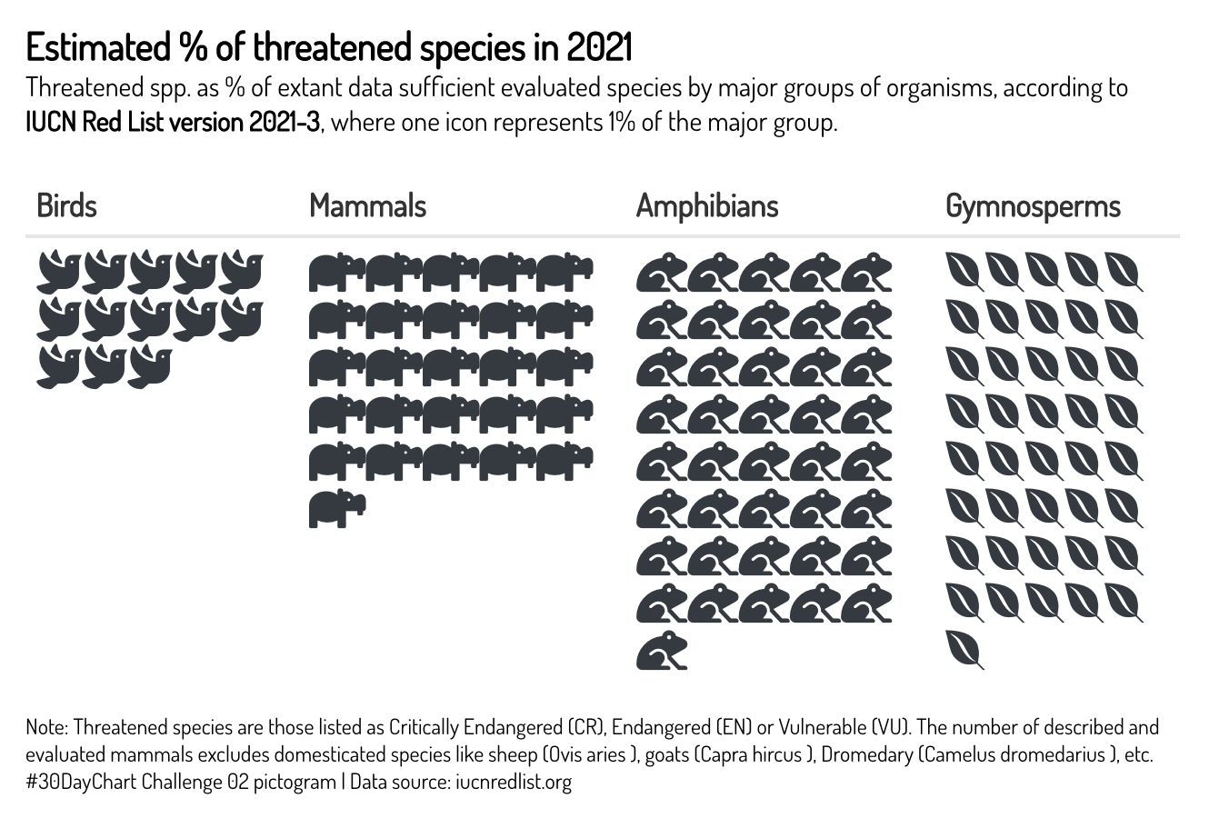

Adding an icon legend

There are a few custom icon legends available within {reactablefmtr} that can be used to describe the icons used in the table:

cars <- mtcars %>%
  rownames_to_column(var = 'model') %>% 
  select(c(model,cyl,am,hp,qsec)) %>%
  mutate(rank = rank(qsec)) %>% 
  relocate(rank, .before = 'model') %>% 
  mutate(medals = case_when(
    rank <= 3 ~ 'medal',
    TRUE ~ ''
  ),
  medal_colors = case_when(
    rank == 1 ~ '#D6AF36',
    rank == 2 ~ '#D7D7D7',
    rank == 3 ~ '#A77044',
    TRUE ~ 'grey'
  )) %>% 
    mutate(transmission = case_when(
    am == 0 ~ 'Automatic',
    am == 1 ~ 'Manual',
    TRUE ~ 'Missing'
  )) %>% 
  select(-am) %>%
  select(c(rank,medal_colors,medals,model,transmission,hp,cyl,qsec)) %>%
  filter(rank <= 11)

reactable(cars,
  theme = nytimes(centered = TRUE, font_color = '#444444'),
  compact = TRUE,
  defaultSortOrder = 'asc',
  defaultSorted = 'qsec',
  pagination = FALSE,
  showSortIcon = FALSE,
  columns = list(
    model = colDef(
      name = 'MODEL / TRANS.',
      maxWidth = 150,
      cell = merge_column(
        data = cars,
        merged_name = 'transmission',
        merged_position = 'below',
        size = 13,
        merged_size = 13
      )
    ),
    cyl = colDef(
      maxWidth = 70, 
      align = 'center',
        cell = icon_assign(
          cars,
          fill_color = 'slategrey',
          empty_color = 'lightgrey',
          empty_opacity = 0.8,
          icon_size = 12
          )
      ),
    hp = colDef(
      align = 'center', 
      maxWidth = 70,
        cell = gauge_chart(
          data = cars,
          size = 1,
          fill_color =  rev(MetBrewer::met.brewer('Troy')), 
          min_value = 50
          )
        ),
    rank = colDef(
      maxWidth = 45,
      cell = icon_sets(
        data = cars,
        icon_ref = 'medals',
        icon_color_ref = 'medal_colors',
        icon_position = 'left',
        number_fmt = scales::number_format(accuracy = 1)
      )
    ),
    transmission = colDef(show = FALSE),
    medals = colDef(show = FALSE),
    medal_colors = colDef(show = FALSE),
    qsec = colDef(
      name = '1/4 mile time',
      align = 'left',
      minWidth = 200,
      format = colFormat(digits = 0),
      cell = data_bars(
        data = cars,
        fill_color = c('#FAFAFA','#E7E7E7','#D3D3D3','#BFBFBF'),
        fill_gradient = TRUE,
        bold_text = TRUE,
        background = 'transparent',
        text_position = 'inside-base',
        text_color = '#222222',
        number_fmt = scales::number_format(accuracy = 0.1, suffix = 's'),
        bar_height = 12,
        min_value = 13,
        max_value = 17.5,
        img = 'https://www.pngkit.com/png/detail/54-544889_45-top-view-of-car-clipart-images-racecar.png',
        img_height = 20,
        img_width = 25
      )
    )
  )
) %>% 
  add_title(
    title = html("Top 10 Fastest Cars <i class='fas fa-flag-checkered'></i>"),
    font_color = 'black',
    margin = reactablefmtr::margin(t=0,r=0,b=2,l=0)
  ) %>% 
  add_subtitle(
    subtitle = "Motor Trend Car Road Tests (mtcars data set)",
    font_size = 18,
    font_color = '#222222',
    margin = reactablefmtr::margin(t=0,r=0,b=4,l=0)
  ) %>% 
  add_icon_legend(
    icon_set = 'medals'
  )

Top 10 Fastest Cars

Motor Trend Car Road Tests (mtcars data set)

Bronze Silver Gold

Embed images

You can embed images directly from the web via the background_img() and embed_img() functions.

embed_img() embeds an image to the foreground of the cell. background_img() embeds an image to the background of the cell.

library(nflfastR)
library(nflreadr)

nflreadr::load_rosters(2021) %>% 
  dplyr::filter(position == "QB") %>% 
  filter(full_name %in% c("Patrick Mahomes","Tom Brady","Aaron Rodgers","Matthew Stafford","Joe Burrow","Josh Allen","Lamar Jackson","Justin Herbert")) %>% 
  left_join(teams_colors_logos, by = c('team' = 'team_abbr')) %>% 
  select(full_name, headshot_url, team_logo_espn, jersey_number, position, team, height, weight, years_exp, college) %>% 
  mutate(height = paste0(floor(as.numeric(height)/12), "'", (as.numeric(height)/12 - floor(as.numeric(height)/12))*12, "''")) %>%
  reactable(
    theme = fivethirtyeight(centered = TRUE),
    defaultColDef = colDef(align = 'center'),
    columns = list(
      team_logo_espn = colDef(show = FALSE),
      full_name = colDef(maxWidth = 200, name = 'Name'),
      jersey_number = colDef(name = '#', maxWidth = 50),
      position = colDef(name = 'Position'),
      college = colDef(name = 'College'),
      years_exp = colDef(name = 'Experience'),
      height = colDef(name = 'Height'),
      headshot_url = colDef(name = '', minWidth = 150, 
        cell = embed_img(
          height = 100, 
          width = 135
        ),
        style = background_img(
          data = ., 
          height = '140%',
          img_ref = 'team_logo_espn'
        )
      )
    )
  )

Data visualizations

When using {reactablefmtr}, remember that you are not just limited to creating tables. By hiding some of the table elements, you can convert your table to a data visualization like the one shown below:

# read in data
parks <- readr::read_csv('https://raw.githubusercontent.com/rfordatascience/tidytuesday/master/data/2021/2021-06-22/parks.csv')

# remove dollar sign and convert to numeric
parks_df <- parks %>% 
  filter(year == 2020) %>% 
  mutate(spend_per_resident_data = parse_number(spend_per_resident_data)) %>% 
  select(city, spend_per_resident_data)

# top 10 spend/resident
top10 <- parks_df %>% 
  top_n(10, spend_per_resident_data) %>% 
  mutate(spenders = 'Top 10 spenders')

# join with bottom 10 spend/resident
parks_df %>% 
  top_n(-10, spend_per_resident_data) %>% 
  mutate(spenders = 'Bottom 10 spenders') %>% 
  rbind(top10) %>% 
  mutate(spender_pal = case_when(
    spenders == 'Top 10 spenders' ~ '#feb98d',
    spenders == 'Bottom 10 spenders' ~ '#000000'
  )) %>% 
  arrange(desc(spend_per_resident_data)) %>% 
  reactable(
    data = .,
    pagination = FALSE,
    theme = void(
      cell_padding = 1, 
      header_font_size = 0, 
      font_color = '#000000', 
      font_size = 15,
      centered = TRUE
      ),
    columns = list(
      spenders = colDef(show = FALSE),
      spender_pal = colDef(show = FALSE),
      city = colDef(maxWidth = 140, align = 'right'),
      spend_per_resident_data = colDef(
        cell = data_bars(
          data = ., 
          fill_color_ref = 'spender_pal', 
          background = 'transparent',
          text_position = 'outside-end',
          bar_height = 22,
          max_value = 450, 
          number_fmt = scales::number_format(prefix = '$'))
        )
      )
  ) %>% 
  add_title(
    title = 'Park Spending Per Resident',
    font_size = 26
  ) %>% 
  add_subtitle(
    subtitle = 'Those who spent the most and least out of the 100 most populated cities. The national median is $89 per capita as of 2020.',
    font_size = 22, 
    font_weight = 'normal',
    margin = reactablefmtr::margin(t=4,r=0,b=0,l=0)
    ) %>% 
  add_subtitle(
    subtitle = 
    tags$div(htmltools::tagAppendAttributes(shiny::icon('square'), style = 'color: #000000; font-size: 14px'), 'Bottom 10 spenders',
             htmltools::tagAppendAttributes(shiny::icon('square'), style = 'color: #feb98d; font-size: 14px'), 'Top 10 spenders'),
    font_size = 15, 
    font_weight = 'normal',
    margin = reactablefmtr::margin(t=12,r=0,b=6,l=0)
    ) %>%
  add_source(
    font_size = 15, 
    source = 'Data: The Trust for Public Land | Original Viz: Bloomberg | Re-created Viz: {reactablefmtr}',
    margin = reactablefmtr::margin(t=25,r=0,b=0,l=0)
    )

Park Spending Per Resident

Those who spent the most and least out of the 100 most populated cities. The national median is $89 per capita as of 2020.

Bottom 10 spenders Top 10 spenders

Data: The Trust for Public Land | Original Viz: Bloomberg | Re-created Viz: {reactablefmtr}